How should I allocate spend across marketing channels like TV and paid search? If you’re managing a company’s marketing budget, this may be the most essential question to maximize profit or revenue given limited spend. There’s three typical ways to answer it scientifically:
- Top down: take all of your data on which days (/weeks, etc.) you spent on which channels, and when your revenue came in. Then, use a media mix model (MMM or marketing mix model) to determine the expected efficiency of each channel across a variety of spend levels.
- Bottom up: use as granular data as possible on which customers saw which ads, and if/when those customers converted. Use a multi-touch attribution model (MTA or attribution) to determine which ads drove each purchase/conversion, then sum your results by channel to see how valuable each one is.
- Lift testing: run isolated experiments such as geo tests, which give you the strongest read on how much incremental value a channel provides. However, it’s expensive to run (think of the opportunity cost in your control geos), especially given how many channels there are and how quickly results become stale.
At Wayfair, we used MTA to get hyper granular results, which let us optimize our marketing channels down to the individual performance of 20m ads across 870 product classes, by using Bayesian bidding models. I really enjoyed using it to analyze the customer journey at a deep level, like measuring which website touchpoints led to a customer purchase. However, attribution is not good at comparing across marketing categories such as online vs. offline, because these categories generate different quantities of touchpoints. For example, paid search like Google Ads pairs fantastically with attribution because each click generates a touchpoint; whereas traditional TV advertising can be valuable, but leads to few associated touchpoints.
In contrast, MMM uses only high level data from each channel, so it can capture results from any channel regardless of the touchpoints acquired. Its downside is that it only provides a 10,000 foot view of the channel’s efficacy over time. This still has significant benefits: it’s kind of like a lift test for every channel that you can run every day, but a lift test that also shows the spend-response curve, answering questions like “if we spend another $10K on Facebook, how many conversions can we expect to receive?”. This makes it a powerful tool for determining budget allocations, building financial forecasts, and providing performance insights on seasonal trends, market conditions, and other factors affecting marketing efficacy.
How to run Media Mix Modeling (MMM)
Theory
- Define Objectives and Scope, and Build Alignment
- Identify the primary goals of the media mix model (e.g., ROI measurement, budget allocation). What questions do you want to answer? Marketing and Data should both be a part of this process, since the model is useless if Marketing doesn’t test it.
- Based on 1-1, you’ll need to choose an optimization goal based on your business. This will most likely be revenue or conversions.
- Collect Data
- Gather spend data on marketing spend and performance across all relevant channels (e.g., TV, radio, digital ads, social media). Depending on your modeling approach, you may need impressions as well.
- Collect external data that might impact marketing performance, such as economic indicators, seasonality, and competitive actions.
- CLEAN and VALIDATE your data! You can test impressions against spend, and test spend against APIs and other business units (e.g. Finance)
- Data Integration and Preprocessing
- Integrate the sources above into a unified dataset. Handle missing values, outliers, and any data anomalies.
- Exploratory Data Analysis (EDA)
- Perform EDA to understand the relationships and patterns in the data. Visualize trends, seasonality, and correlations between marketing activities and performance metrics.
- Select and Build the Model
- Choose appropriate modeling techniques (e.g., regression analysis, time-series analysis, machine learning models). You can also consider a pre-built package like Cassandra or Meta’s Robyn. If you’ve really got the $$, you can purchase SaaS MMM as well.
- Build and validate the model, accounting for interaction effects and the diminishing returns of each channel.
- Currently Meta’s Robyn model doesn’t account for interaction effects. Options to do so could include adding interaction terms to your regression, or using a tree based model.
- Robyn models diminishing marginal returns by combining saturation curves and a hill function
- Validate your model
- Statistical tests and performance metrics: R-squared should ideally be >0.80, mean absolute error will depend on your modeled outcome.
- Assumptions in the model should conform to Marketing’s expectations, e.g. if you’re using a decay function, the decay for TV should be slower than for SEM.
- Use the model to simulate different budget allocation scenarios and their potential impact on performance
- Optimize the media mix by reallocating budgets to channels with the highest ROI potential
- Test the updated allocation
- Run a power analysis to determine the minimal amount of spend you’d need to reallocate to be 90% confident you’ll observe an effect
- Make large enough changes to the budget and observe the effects on your dependent variable. Create a feedback loop to take learnings and reapply them to both MMM and spend
Practice
I’m using an example dataset called ‘df’, a Python Pandas dataframe, which contains a couple hundred weeks of spend data and the conversions they generated. The 3 channels are ‘TV’, ‘radio’, and ‘newspaper’, and conversions are ‘sales’, in $ spent and # sold, respectively.* For this post, the ETL and data cleaning steps are already complete. They’re available in the full python script.
| TV | radio | newspaper | sales | |
|---|---|---|---|---|
| 0 | 230.1 | 37.8 | 69.2 | 22.1 |
| 1 | 44.5 | 39.3 | 45.1 | 10.4 |
| 2 | 17.2 | 45.9 | 69.3 | 9.3 |
| 3 | 151.5 | 41.3 | 58.5 | 18.5 |
| 4 | 180.8 | 10.8 | 58.4 | 12.9 |
*An assumption given that channel spend is 10x sales, which would be unprofitable if both were in $
EDA
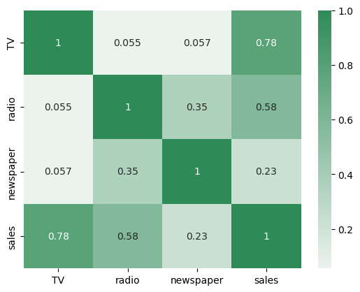
Step one when working with a new dataset is always to understand what you’re working with. I’ll create a correlation matrix and pair plot to see how these features are related to each other.
corr = df.corr()
sns.heatmap(corr, xticklabels = corr.columns, yticklabels = corr.columns, annot = True, cmap = sns.light_palette(color='seagreen', as_cmap=True))

It looks like TV is most heavily correlated with sales, and could be our best bet for driving performance. Also, radio and newspaper tended to be used together more often than any other pair of channels, even though so far newspaper isn’t very correlated with sales. Perhaps we’ll be able to trim our newspaper usage.
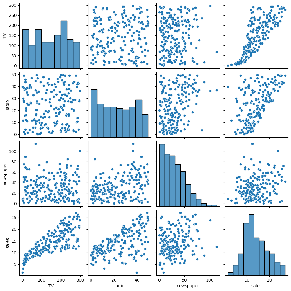
Next let’s make a pair plot to show a) scatterplots of the relationship between different variables, and b) histograms along the diagonal that show the frequency of each value.
# How simple is this? Python is amazing
sns.pairplot(df)

There’s a lot to take away from this. Starting on the right with channels’ relationship with sales, it looks like TV has a clear relationship with sales, especially when considering no TV vs. some TV, while radio may have a looser relationship, and newspaper looks totally irrelevant given its random distribution. TV looks like it could have an exponential relationship, at least at first. Next, it looks like newspaper’s data is skewed to the left, with most weeks spending <$50 but some weeks spending close to $100; we may want to correct that using a transformation like Box Cox. Lastly, there’s no obvious trend between the 3 independent variables.
Model selection, training, and testing
Let’s keep this really simple. The model building process looks like this:
- Identify models that fit the problem and the data at hand
- Build said models, and measure how accurately they can predict your test data
- Choose the model that performed the best and productionize it
We’re working with a regression problem with a continuous dependent variable and 3 independent variables, so our two main choices are a linear model or a tree-based model. Let’s dive into the most common algorithms we can consider:
- “Linear” models (called so since they’re variants of linear regression, but some of them can handle non-linear data)
- Multiple linear regression - this model fits the scenario I described above, but our data isn’t linear, so it’s not likely to perform very well. However, if we adjust our data by e.g. taking the log of the dependent variable, we may be able to fit a line to it; this would be called a log-linear model and is likely worth trying since it’s so easily interpretable if it works.
- Ridge & lasso regression - these regularization adjustments to linear regression correct for collinear data and shrink coefficients. Since in this toy example our variables aren’t very highly correlated, these are likely to be of less use; but since typically marketing channels like Facebook and TikTok are highly correlated, I’d recommend this approach. Meta’s Robyn for instance uses a ridge regression, i.e. linear regression with L2 regularization.
- Polynomial regression - now we’re talking. This is linear regression but as applied to non-linear data. Sounds promising!
- Tree-based models
- Decision tree - sure we could use one decision tree, but whoever uses one when the whole forest is available? And it’s still environmentally friendly
- Random forest - these models are highly accurate and are not particularly prone to overfitting. Since our data complexity is low, the only major disadvantage is that they’re not very interpretable
- Gradient boosting and XGBoost - these models can be even more accurate than random forests, although they’re sensitive to outliers and can overfit. Our data doesn’t have too many outliers though, except arguably on days where spend was close to 0, so this looks promising
If I were getting paid to solve this problem, I’d test out log-linear regression, polynomial regression, random forests, gradient boosting, and XGBoost. But I’m not, so I tried log-linear regression and random forests, so that I’d get results from both the “linear” and tree-based models. Spoiler alert: random forests won, so let’s focus on that. (Again, the full analysis is available here).
# create our X and y variables from our df. y is simply the sales data
X = df.iloc[:,0:3]
y = df.iloc[:,3]

# create a randomized split of training and testing data
X_train, X_test, y_train, y_test = train_test_split(X, y, test_size=.25, random_state=7)
# create the random forest model and train it
rf_model = RandomForestRegressor(random_state=7)
rf_model.fit(X_train, y_train)
# create predictions using our training data, then save them
pred = rf_model.predict(X_test)
rf_results = pd.DataFrame({'actual': y_test, 'pred':pred})

# evaluate our results with a plot of predictions vs. actuals. Sort by actual sales for readability
rf_results.sort_values(inplace=True,by='actual')
rf_results.reset_index(inplace=True, drop=True)
plt.plot(rf_results.index.values, rf_results.actual.values, color='b', label='actual')
plt.plot(rf_results.index.values, rf_results.pred.values, color='r', label='predicted')
plt.xlabel('Observation #')
plt.ylabel('Sales')
plt.legend(loc='upper left')
plt.show()

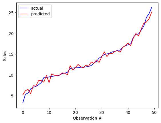
The plot above shows our random forest’s predictions for sales vs. the test data (which we created by splitting our data set into 25% test data and 75% training data). It looks pretty reasonable! Let’s look at some aggregate measures of error.
# random forest model error
rf_actual = rf_results['actual'].values
rf_pred = rf_results['pred'].values

print(metrics.mean_absolute_error(rf_actual, rf_pred))
print(metrics.mean_squared_error(rf_actual, rf_pred))
# taking the square root gets us root mean squared error
print(np.sqrt(metrics.mean_squared_error(rf_actual, rf_pred)))
MAE = 0.73
MSE = 1.03
RMSE = 1.02
This was a significant improvement over e.g. the log linear model error, which had a mean average error of 1.23, and a mean squared error of 2.95. This means that while the random forest had about half to two-thirds as much error on average (0.73 vs. 1.23) it had just one third as much error when using a metric that punishes outliers (1.03 vs. 2.95). (Refresher on types of error here).
Budget optimization
Now that we have a working model, what does it tell us about how should we spend our marketing budget? The ideal process for this would use a multi-armed bandit test to run through the following process:
- Feed X values into the model
- Record the output y, and repeat until you’ve maximized y
Given the dataset, there are some open questions.
- How much is a sale/conversion worth? We know marketing spend, but not marketing revenue or profit
- What are the goals of the business right now? Maximize growth by focusing on revenue or customer acquisition? Generate profits to appease stakeholders or pay off debt obligations?
- Are there budget or efficiency constraints, or are we free to spend as much as needed to hit the business goal? Without these pieces of business context, we can’t truly optimize the budget. What we can do is figure out optimal budget allocations at different levels of spend. What levels of spend should we focus on?
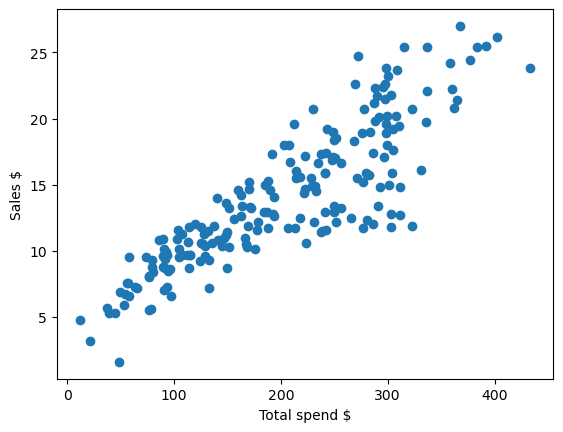
Looking at our training data, we have weekly spend figures between about $0 and $400. Random forests perform worse at extrapolating than interpolating, so let’s limit our results to this range. We’ll seek to maximize sales within that budget.
# Plot total spend vs. sales in our training data
# Note that there's also a clear relationship between spend and sales
plt.scatter(X.sum(axis=1),y)
plt.xlabel('Total spend $')
plt.ylabel('Sales $')

As mentioned, a multi-armed bandit test would be the ideal way to find the optimal allocation. But given that it’s a 3-variable problem, we can actually calculate a solution by trying all possible values (in multiples of 5).
# create 500K options to test
import itertools
tv = list(range(0-ns, 401-ns, 5))
radio = list(range(0-ns, 401-ns, 5))
np = list(range(0-ns, 401-ns, 5))
s = [tv, radio, np]

# run each budget allocation through our random forest
y_three = rf_model.predict(trials_three)

# create dataframe and pull the maximum sales we can generate; and of those, the minimum spend
trials_three = pd.DataFrame(list(itertools.product(*s)), columns=['TV','radio','newspaper'])
trials_three['total_spend'] = trials_three.sum(axis=1)
trials_three['sales'] = y_three
max_alloc = trials_three.query('sales == sales.max()')
max_alloc.query('total_spend == total_spend.min()')
The Verdict
There we have it: in experiment 361,670 we found our ideal allocation. 275 to TV, 50 to radio, and 25 to newspaper, assuming we want to maximize sales but constrain our budget to be <$400. I’d recommend shifting spend from radio and newspaper to TV to accomplish this, ideally in an A/B testing framework, such as by running a geographical study using the new approach as the treatment.
| TV | radio | newspaper | total_spend | sales | |
|---|---|---|---|---|---|
| 361670 | 275 | 50 | 25 | 350 | 26.386 |
Next steps for model development
With limited time, there were plenty of optimizations I skipped over that could be used to refine our answer.
- In my opinion the largest gap is that there’s no accounting for effect over time: each week is treated as separate. In reality, TV advertising one week likely increases conversions for the next few weeks as well. To account for this, we’d want to use Bayesian methods to account for carryover and shape effects, as described here.
- Similarly, there’s no accounting for seasonality, and spend in certain areas may work better some weeks/months than others. Getting time series data could let us add that as a feature to analyze.
- We didn’t optimize the RF’s hyperparameters; doing so can lead to increased predictive accuracy.
- We could have used sampling to find the confidence and prediction intervals for the model. This would tell us how confident each estimate is. Here is one methodology to do so.
- Feature selection: while testing model error, or once we’ve selected a model, it’s often helpful to prune features that aren’t contributing to its predictive power. However, given that we only have 3 variables, and each has an effect on sales, I elected to keep all three in the model.
Overall takeaways
In order to make a recommendation, we had to make some assumptions about the business’ needs and the value of conversions/sales. In a real business setting, understanding the goals of the business and the value of our conversions would be some of the first steps we’d need to take while planning out our analysis. But now that we have a recommendation - move about 80% of spend to TV, while keeping both radio and newspaper but as smaller channels - we’d want to run A/B testing to validate these results. Since there’s still improvements to be made in the model, we’d want to keep this test small and cheap, to validate investing more time into our predictions; or perhaps, depending on the exact cost of that A/B test, run it after building seasonality and the impact of spend over time into our model.
In sum, this media mix model was a fairly quick way to identify that the business is likely not investing enough in TV. And really, it should consider adding a 4th, 5th, or 10th marketing channel!