This week I built a classifier that determines whether Pitchfork’s album reviews qualify for “Best New Music” based on the review text. I rely pretty heavily on Pitchfork to find new music and better understand what I’m listening to, and analyzing the results of this classifier helped me investigate a few questions about how the site’s reviews work:
- What does Pitchfork value in an album? (Spoiler: jazz)
- Where does Pitchfork have biases or blind spots?
- What kind of creative language do reviewers use to describe great or terrible albums?
How does the classifier work?
It scrapes review text from Pitchfork’s website, then creates a matrix of how many times each word appears in each review, which it uses to train a naive Bayes classification algorithm to predict whether the album’s score will be 8.0 or higher. With this algorithm, we can model which words best signify an excellent album. In future iterations, incorporating word embedding would allow the model to learn the meaning behind the words, rather than just analyzing individual words in a vacuum, which would improve the classifier’s accuracy by allowing it to understand how words that can be positive or negative in different contexts are used.
Scraping Pitchfork for Reviews
The first step is to gather our data. I started with a matrix of review links and metadata from github user Meddulla. Then, by pulling all the html from each webpage, I add the review text itself to the dataframe.
#import the artists and albums from 'meddulla's github page
pitchfork_data = pd.read_csv(
    'https://gist.githubusercontent.com/meddulla/8277139/raw/f1595d50cada910d082bc1dfd8ef47ff49910cb3/pitchfork-reviews.csv',
           sep = ',')
pitchfork_data.head()

# a note on scraping pitchfork: according to their robots.txt file, scraping is allowed,
# as long as users aren't scraping any of their search pages.
| artist | album | score | reviewer | url | |
|---|---|---|---|---|---|
| 0 | Burial | Rival Dealer EP | 9.0 | Larry Fitzmaurice | http://pitchfork.com/reviews/albums/18820-buri... |
| 1 | The Thing | BOOT! | 7.7 | Aaron Leitko | http://pitchfork.com/reviews/albums/18735-the-... |
| 2 | Lumbar | The First And Last Days Of Unwelcome | 7.7 | Grayson Currin | http://pitchfork.com/reviews/albums/18705-lumb... |
| 3 | Bryce Hackford | Fair | 7.0 | Nick Neyland | http://pitchfork.com/reviews/albums/18789-bryc... |
| 4 | Waka Flocka Flame | DuFlocka Rant 2 | 7.1 | Miles Raymer | http://pitchfork.com/reviews/albums/17760-waka... |
#input: urls in a pandas series format
#output: review text for each of those links as an array of strings
from bs4 import BeautifulSoup

def get_multiple_reviews(urls):
    if isinstance(urls, pd.Series):
        review_text = []

        for link in urls:
            #pull url html into a beautifulsoup object
            try:
                r = requests.get(link)
                soup = BeautifulSoup(r.text, 'lxml')
                #pull all paragraph tags/contents with soup.findAll, and then put the text into one string
                review_text.append('\n\n'.join(map(str, [i.text.lower() for i in soup.findAll('p')])))
            except Exception:
                review_text.append(np.nan)
        return review_text

    else:
        print('Check inputs - confirm they\'re in pd.Series format')
        return
##this code executes the review scraping function. since scraping 5000 reviews takes a while, I've saved it as a csv file.
#sample_df = pitchfork_data.sample(5000)
#sample_df['review'] = sample_reviews_merged
#sample_df.to_csv('C:\\Users\\Matt\\Documents\\Python_Scripts\\CS109_Zips\\2013-homework\\HW Practice\\pitchfork_reviews.csv')
#pull in scraped data saved as a csv for convenience
sample_df = pd.read_csv(
    'C:\\Users\\Matt\\Documents\\Python_Scripts\\CS109_Zips\\2013-homework\\HW Practice\\pitchfork_reviews.csv',
     sep=',', encoding = 'latin-1', index_col = 'Unnamed: 0')
sample_df.head()
| artist | album | score | reviewer | url | review | |
|---|---|---|---|---|---|---|
| 4631 | August Born | August Born | 7.3 | Matthew Murphy | http://pitchfork.com/reviews/albums/484-august... | drag city-issued collaboration between six org... |
| 4034 | Deerhunter | Cryptograms | 8.9 | Marc Hogan | http://pitchfork.com/reviews/albums/9824-crypt... | best new music\n\nthis atlanta five-piece's sh... |
| 3224 | Unicycle Loves You | Unicycle Loves You | 6.5 | Ian Cohen | http://pitchfork.com/reviews/albums/12057-unic... | despite making ebullient indie pop, this chica... |
| 2212 | Flying Lotus | Cosmogramma | 8.8 | Joe Colly | http://pitchfork.com/reviews/albums/14198-cosm... | best new music\n\nthe l.a. producer's head mus... |
| 4989 | Skalpel | Skalpel | 7.2 | Jonathan Zwickel | http://pitchfork.com/reviews/albums/7768-skalpel/ | ninja tune exports skalpel cut up dusty 50s an... |
print('min/mean/max: ',pitchfork_data.score.min(), '/', pitchfork_data.score.mean(), '/', pitchfork_data.score.max())
print('# reviews: ',len(sample_df))
min/mean/max:  0.0 / 6.955978497748127 / 10.0
# reviews:  5000
Clean the data
If any of the links are dead, our scraper will import a NaN, so let’s clean those up.
print('NA values before cleaning: ',sum(sample_df.review.isnull()))
sample_df = sample_df.reset_index(drop=True)
sample_df.drop(sample_df.index[sample_df[sample_df.review.isnull()].index.values], axis=0, inplace=True)
print('NA values now: ',sum(sample_df.review.isnull()))
NA values before cleaning:  2
NA values now:  0
Data Exploration
Visualizing the Reviewers
print('# of reviews: ', len(sample_df))
print('# of reviewers: ', len(sample_df.reviewer.unique()))
# of reviews:  4998
# of reviewers:  234
#Histogram to look at the spread of reviewers
plt.title('How Prolific are the Reviewers?')
plt.xlabel('Quantity of Reviews')
plt.ylabel('Number of Reviewers')
plt.hist(sample_df.groupby('reviewer').review.count(), bins=40)
plt.show()
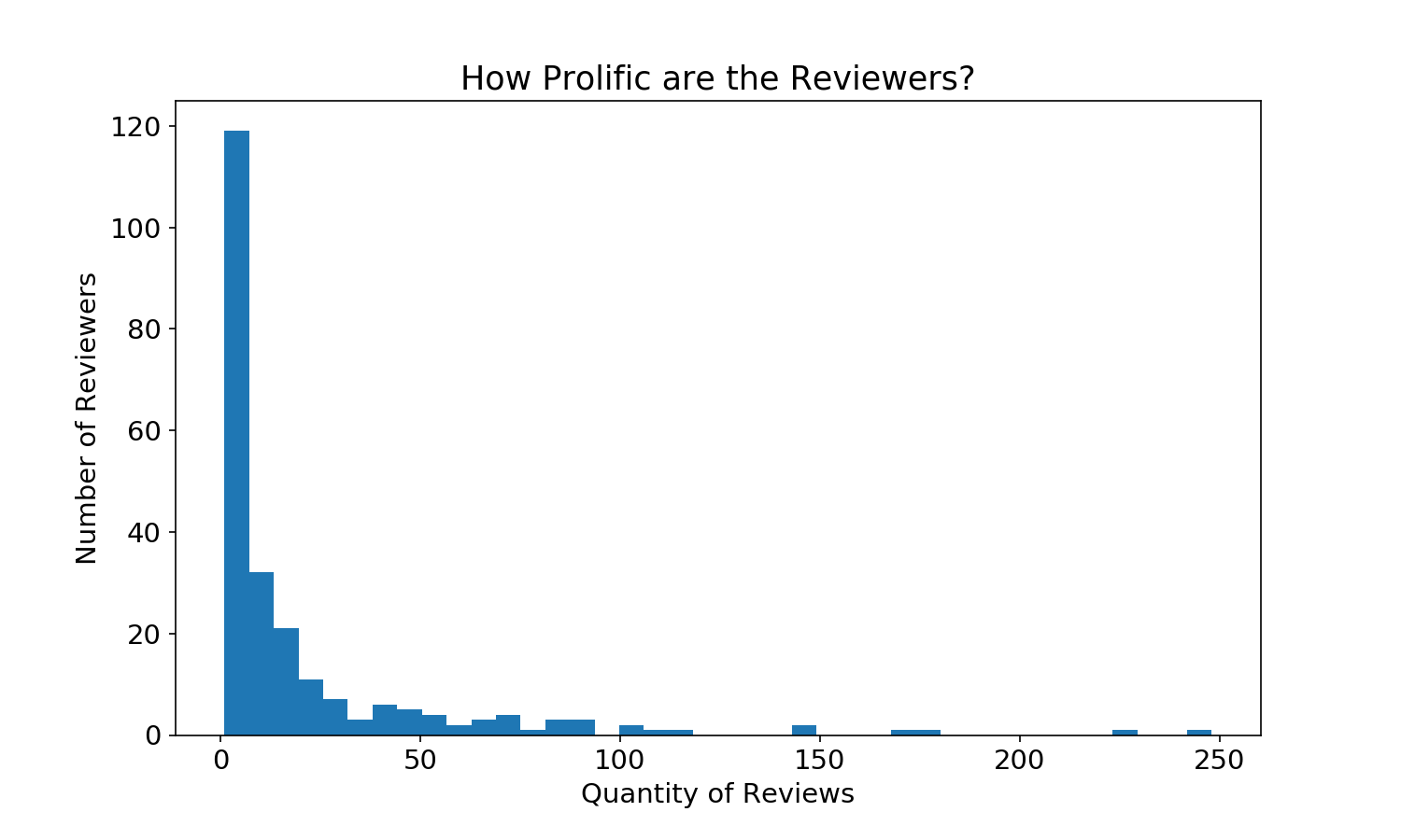
top_5_reviewers = sample_df.groupby('reviewer').review.count().nlargest(5)
print('The 5 most prolific reviewers:\n', top_5_reviewers)
The 5 most prolific reviewers:
 reviewer
Joe Tangari           248
Stephen M. Deusner    228
Ian Cohen             176
Brian Howe            169
Mark Richardson       149
Name: review, dtype: int64
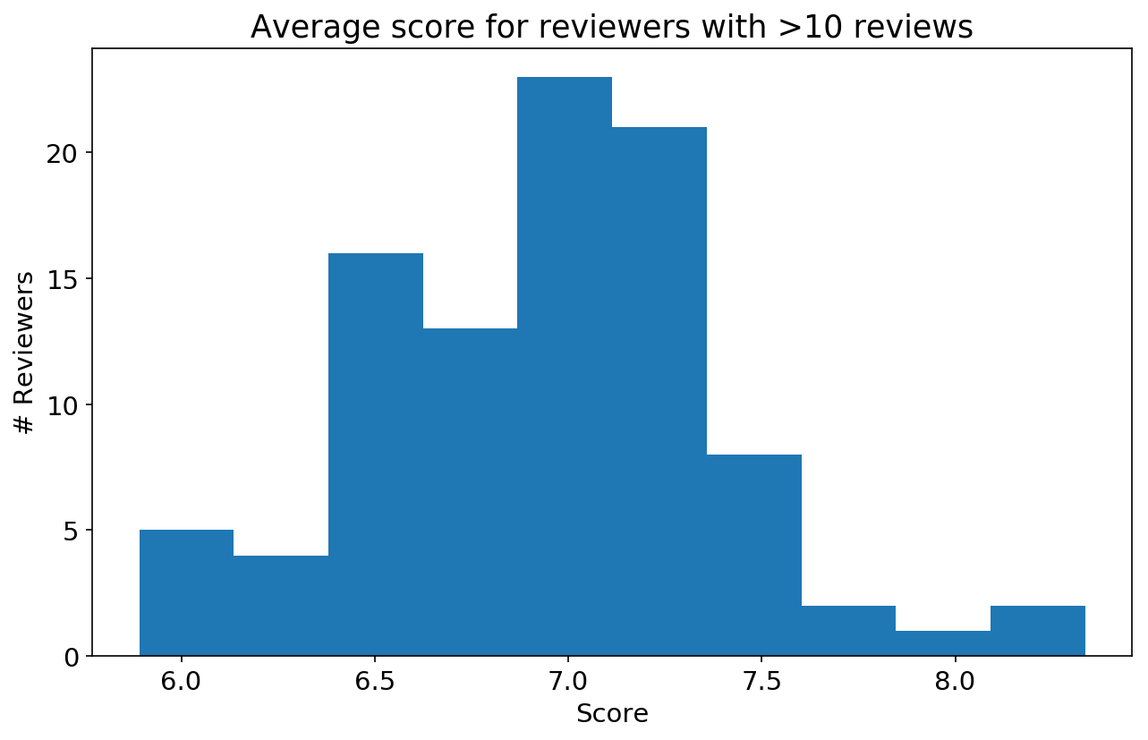
#pull the names of all reviewers with >n reviews
#use that to get average reviews for relatively prolific reviewers
floor_score = 10
df_count = sample_df.groupby('reviewer').count()
df_mean = sample_df.groupby('reviewer').mean()
plt.title('Average score for reviewers with >%i reviews' %floor_score)
plt.ylabel('# Reviewers')
plt.xlabel('Score')
plt.hist(df_mean[sample_df.groupby('reviewer').count().review>floor_score].score)
plt.show()
Visualizing the Reviews
Vectorizing the data will let us see which words appear most frequently.
#import vectorizer and fit it to our data
from sklearn.feature_extraction.text import CountVectorizer
vectorizer = CountVectorizer()
vectorizer.fit(sample_df.review)

#assign vectorizer data to an array
x = vectorizer.transform(sample_df.review)
x = x.toarray()
print('number of words in the dataframe: ', len(vectorizer.get_feature_names()))
words = pd.DataFrame({'word':vectorizer.get_feature_names(),'freq':x.sum(axis=0)})
print('20 highest frequency words: ', [i for i in words.nlargest(20, 'freq').word.values])
number of words in the dataframe:  71027
20 highest frequency words:  ['the', 'of', 'and', 'to', 'in', 'that', 'it', 'is', 'on', 'with', 'as', 'for', 'but', 'his', 'like', 'you', 'from', 'this', 'their', 'an']
print('# words that appear once: ', words[words.freq == 1].freq.count())
print('The most common word appears ', words.freq.max(),' times')
print('Most common word: ', words[words.freq == words.freq.max()].values[0][1])
# words that appear once:  24334
The most common word appears  177053  times
Most common word:  the
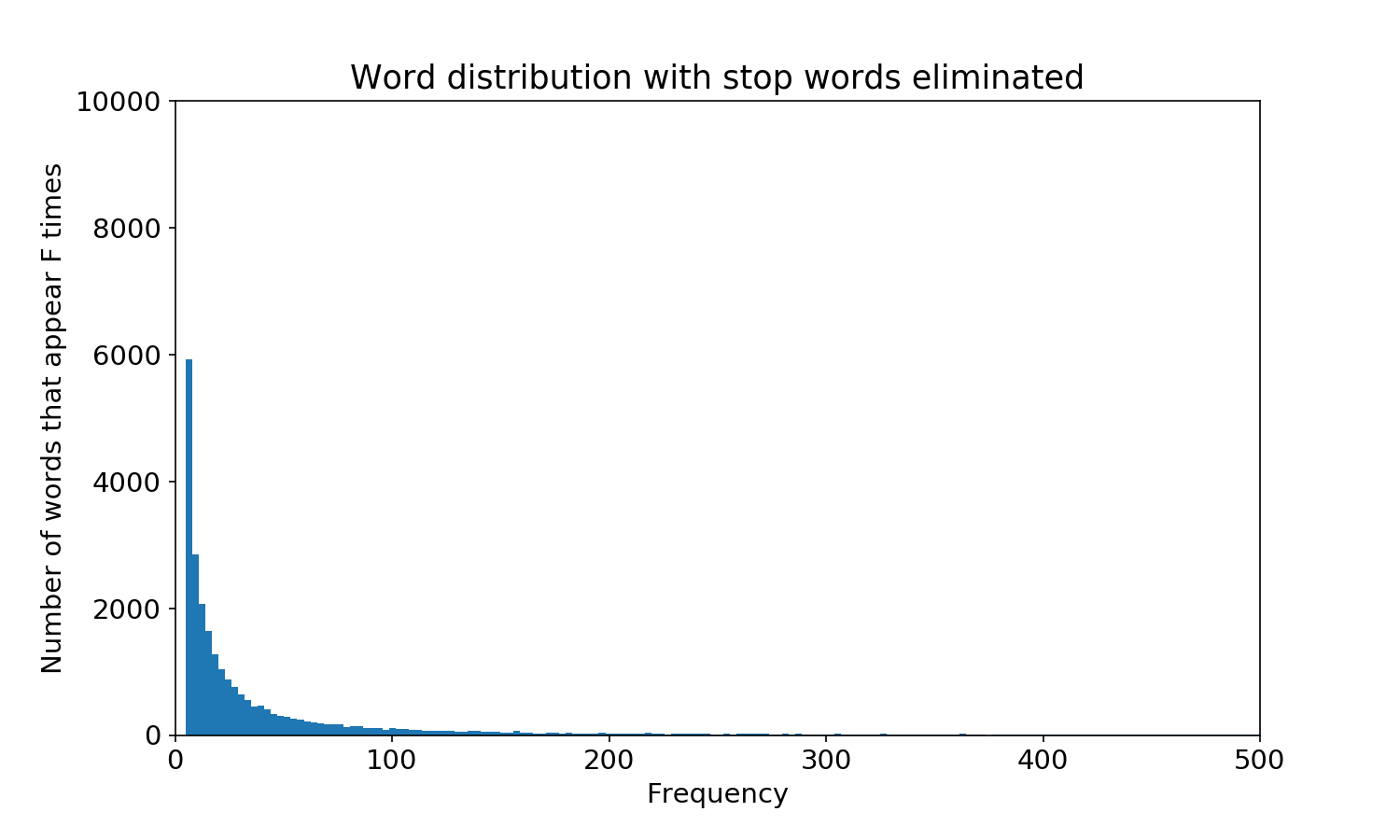
Stop words like ‘the’ aren’t very meaningful, and words that appear once in a blue moon are not generalizable, so let’s add some limits to the frequency of words
We’ll use a gridsearch to pick the ideal vectorization parameters later; for now let’s just try 1e-03 and 0.1 for our min and max.
vectorizer = CountVectorizer(min_df = 1e-03, max_df = 0.1)
vectorizer.fit(sample_df.review)
x = vectorizer.transform(sample_df.review)
x = x.toarray()
len(vectorizer.get_feature_names())
words = pd.DataFrame({'word':vectorizer.get_feature_names(),'freq':x.sum(axis=0)})
print('20 highest frequency words: ', [i for i in words.nlargest(20, 'freq').word.values])
20 highest frequency words: ['rap', 'jazz', 'blues', 'singles', 'fire', 'disco', 'hits', 'star', 'fi', 'sun', 'york', 'dream', 'eyes', 'electric', '90s', 'machine', 'organ', 'recordings', 'roll', 'riffs']
print('# words that appear once: ', words[words.freq == 1].freq.count())
print('The most common word appears ', words.freq.max(),' times')
print('Most common word: ', words[words.freq == words.freq.max()].values[0][1])
# words that appear once:  0
The most common word appears  1213  times
Most common word:  rap
plt.hist(words.freq, bins=400)
plt.title('Stop words eliminated')
plt.xlabel('Frequency')
plt.ylabel('Number of words that appear F times')
plt.axis([0,500,0,10000])
plt.show()
print('number of words appearing more than once: ', words[words.freq>1].freq.count())
print('number of words appearing once: ', words[words.freq==1].freq.count())
number of words appearing more than once:  25190
number of words appearing once:  0
That looks great: no more stop words or singletons, and a reasonable distribution of word frequency.
cutoff_score = 8
print('Percent of reviews that are \'best new music\' (>%i.0): ' %cutoff_score, sum(sample_df.score>cutoff_score)
      /sum(sample_df.score>0)*100)
Percent of reviews that are 'best new music' (>8.0): 16.6099659796
Train Classifier
Now that we’ve set up a word matrix with the vectorizer, we can train our naive Bayes classifier on our data. We’ll split our data into training and testing data, optimize our model parameters, and fit the data.
#We'll use this function in our grid search to reconstruct the vectorizer
#critics is the dataframe of reviews, etc.
from sklearn.feature_extraction.text import CountVectorizer

def make_xy(critics, mind=1, maxd=0.99):
    #create y matrix, where y=1 if it's greater than our cutoff score
    bnm = critics.score>cutoff_score
    y = bnm.astype(int).values

    #set up the vectorizer, with terms for min_df and max_df
    vectorizer = CountVectorizer(min_df = mind, max_df = maxd)
    vectorizer.fit(critics.review)
    x = vectorizer.transform(critics.review)
    x = x.toarray()

    return x, y, vectorizer

X, Y, v = make_xy(sample_df, 1, 0.99)

print('Number of words analyzed: ', len(v.get_feature_names()))
print('Average words per article per the min/max_df above: ', np.array([i.sum() for i in X]).mean())
Number of words analyzed:  71021
Average words per article per the min/max_df above:  547.547418968
from sklearn.model_selection import train_test_split
from sklearn.naive_bayes import MultinomialNB
#Select best parameters (min_df, max_df, alpha)

#cs109 parameter selection. gridsearch above
import sklearn.model_selection
#we'll use the area under the roc curve as a metric
from sklearn.metrics import roc_auc_score

#the grid of parameters to search over
alphas = [.1, 0.5, 1, 3, 5, 10, 50]
min_dfs = [1e-4, 1e-3, 1e-2]
max_dfs = [1e-1, 0.2, 0.5]

#Find the best value for alpha and min_df, and the best classifier
best_alpha = None
best_min_df = None
best_max_df = None
max_auc = -np.inf

for a in alphas:
    for min_df in min_dfs:
        for max_df in max_dfs:
            #configure vectorizer
            #vectorizer = CountVectorizer(min_df = min_df, max_df = max_df)
            X, Y, v = make_xy(sample_df, min_df, max_df)

            #split up testing/training
            xtrain, xtest, ytrain, ytest = train_test_split(X, Y, test_size = 0.2)

            #fit the naive bayes model
            nb = MultinomialNB()
            nb.set_params(alpha=a)
            nb.fit(xtrain, ytrain)

            #function below implements kfold validation to find best auc
            y_score = nb.predict_proba(xtest)[:,1]
            nll = roc_auc_score(ytest, y_score)

            #set best params
            if nll > max_auc:
                max_auc = nll
                best_alpha = a
                best_min_df = min_df
                best_max_df = max_df
#show best parameters
print(max_auc, '|', best_alpha, '|', best_min_df, '|', best_max_df)
0.763630952381 | 3 | 0.01 | 0.5
from sklearn.model_selection import train_test_split
from sklearn.naive_bayes import MultinomialNB

#split our data into training data (80%) and testing (20%)
X, Y, v = make_xy(sample_df, best_min_df, best_max_df)
#provide indices so we can examine later
tts_indices = list(range(len(X)))
xtrain, xtest, ytrain, ytest, indices_train, indices_test = train_test_split(
    X, Y, tts_indices, test_size = 0.2, random_state = 10)

#fit the naive bayes model
nb = MultinomialNB(alpha=best_alpha)
nb.fit(xtrain, ytrain)

#test training prediction
print('training accuracy: ', sum(nb.predict(xtrain)==ytrain)/len(ytrain))
print('testing accuracy: ', sum(nb.predict(xtest)==ytest)/len(ytest))
#well this model is most definitely overfit - training performance is much better than testing
#also with just 15% of music as bnm, I'm concerned with 81% accuracy
training accuracy:  0.897698849425
testing accuracy:  0.814
81.6% accuracy sounds good, but given that only about 15% of reviews are for Best New Music, it’s not a great measure of fit. If it misses all of the true positives1, it will fail to classify any music as Best New Music correctly. We’ll construct a better scorer below. 1*http://www.dataschool.io/simple-guide-to-confusion-matrix-terminology/
Testing/scoring the Model
#and that scorer is area under the receiver operating characteristic curve! (aucroc)
from sklearn.metrics import roc_auc_score
y_score = nb.predict_proba(xtest)[:,1]
roc_auc_score(ytest, y_score)
0.74360863095238106
#ROC Curve
from sklearn.metrics import roc_curve, auc
fpr, tpr, thresh = roc_curve(ytest, y_score)
plt.plot(fpr, tpr)
plt.title('ROC Curve')
plt.xlabel('False positive rate (100-specificity)')
plt.ylabel('True positive rate (sensitivity)')
plt.plot(np.linspace(0,1,100),np.linspace(0,1,100))
[<matplotlib.lines.Line2D at 0x162bc36a4e0>]
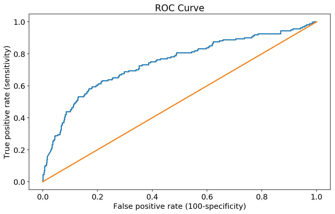
The graph above shows how likely our model is to correctly assign a review of >=8.0 as Best New Music, and a review of <8.0 as not Best New Music. In other words, how well it maximizes true positives while minimizing false positives. See: ROC curve
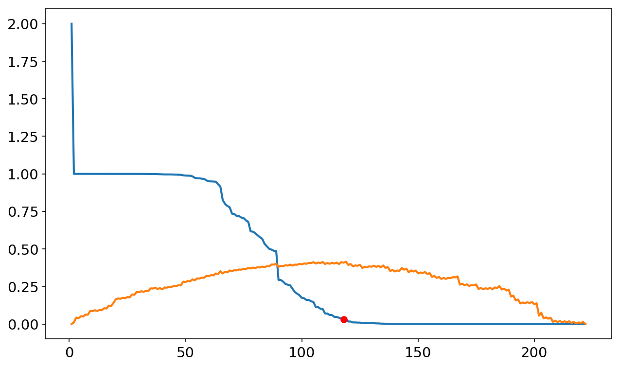
#calculate youden's j and identify the threshold at which it's maximized
youden_j = tpr + (1-fpr) -1
ideal_thresh = thresh[np.where(youden_j == youden_j.max())]
plt.plot(np.linspace(1, len(thresh),len(thresh)),thresh)
plt.plot(np.linspace(1, len(thresh), len(thresh)),youden_j)
plt.plot(np.where(youden_j == youden_j.max()),ideal_thresh,'o', c='r')
print('ideal threshold: ',ideal_thresh)
plt.show()
ideal threshold: [ 0.03175009]
#let's assess whether our model is well-calibrated (i.e. whether its confidence % is about equal to its accuracy %)
hst = plt.hist(nb.predict_proba(xtest)[:,1], bins=20)
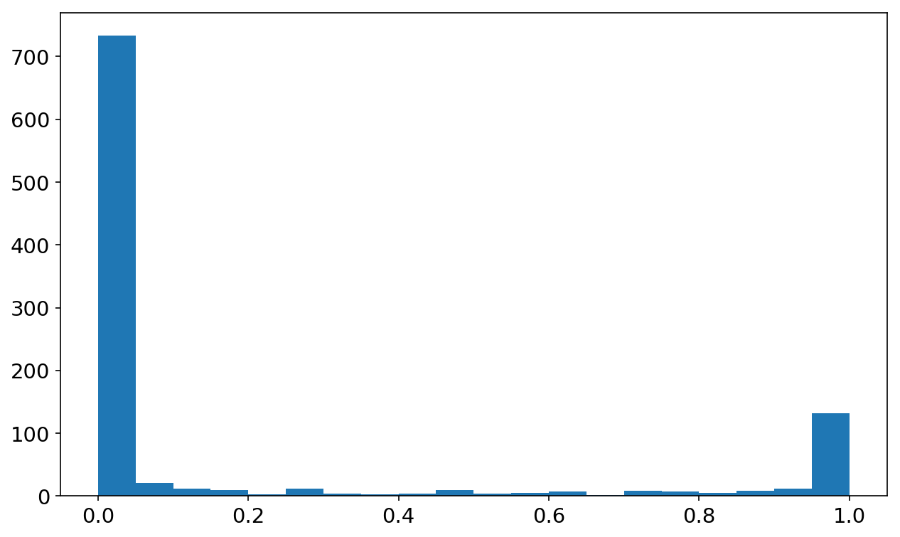
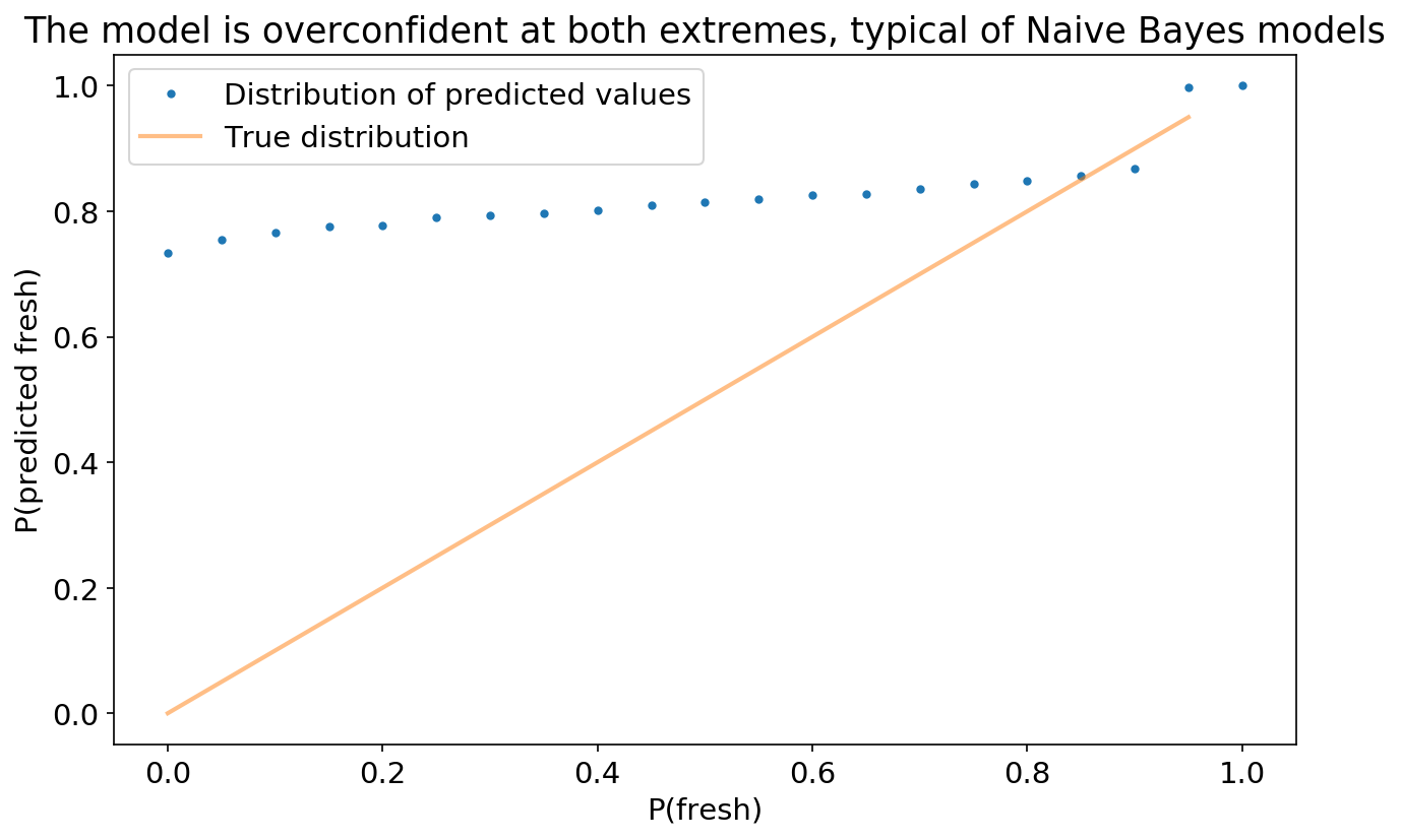
As demo’d above, Naive Bayes tends to push probabilties to 0 or 1, mainly because it makes the assumption that features are conditionally independent, which is not true here.
bin_counts = hst[0]
probabilities = nb.predict_proba(xtest)
digits = np.digitize(probabilities[:,1], hst[1])

#next step is to figure out what % of each bin in our test data is fresh
#so we'll need to assign ytest to bins per digits
binframe = pd.DataFrame({'y':ytest, 'bin':digits})
bnm_prob = binframe.groupby('bin').sum()/binframe.groupby('bin').count()

#number of reviews in each bin divided by the total number of (test) reviews
pct_df = binframe.groupby('bin').count()/binframe.bin.count()

#pct_df won't have the right # of items if the bins aren't nicely distributed, so we'll pad it
ind = list(range(1,len(hst[0])+2))
indy_df = pd.DataFrame({'b':np.zeros(len(ind))}, index=ind)
indy_df = indy_df.join(pct_df)
indy_df = indy_df.max(axis=1)

#plot the cumulative distribution function
plt.xlabel('P(fresh)')
plt.ylabel('P(predicted fresh)')
plt.title('The model is overconfident at both extremes, typical of Naive Bayes models')

#plt.plot(hst[1][:-1], np.cumsum(pct_df.values),'.')
plt.plot(hst[1], np.cumsum(indy_df.values),'.')
plt.plot(hst[1][:-1],hst[1][:-1], alpha=.5)
plt.legend(['Distribution of predicted values', 'True distribution'])
<matplotlib.legend.Legend at 0x162bc10c710>
Looking at incorrect predictions
Let’s look at reviews the model got wrong.
#create list with the indices and test results (w), and split into correct and incorrect
all_pred = list(zip(indices_test,nb.predict(xtest)==ytest))
correct_pred = [i[0] for i in all_pred if i[1] == True]
incorrect_pred = [i[0] for i in all_pred if i[1] == False]

#Where false, the prediction didn't agree with reality
print(sample_df.iloc[incorrect_pred[0],:],'\n\n',
      sample_df.iloc[incorrect_pred[1],:],'\n\n', sample_df.iloc[incorrect_pred[2],:])
artist                                       El Perro Del Mar
album                                        El Perro del Mar
score                                                     8.1
reviewer                                   Stephen M. Deusner
url         http://pitchfork.com/reviews/albums/9087-el-pe...
review      on her second album, swedish singer-songwriter...
Name: 1562, dtype: object

 artist                                                    UGK
album                                       Underground Kingz
score                                                     8.4
reviewer                                          Tom Breihan
url         http://pitchfork.com/reviews/albums/10541-unde...
review      after a six-year absence that found the south ...
Name: 88, dtype: object

 artist                                            Whiskeytown
album                                               Pneumonia
score                                                     8.1
reviewer                                         Ryan Kearney
url         http://pitchfork.com/reviews/albums/8645-pneum...
review      categorization has been widely accepted as a p...
Name: 4177, dtype: object
These scores are each fairly close to 8. That’s encouraging! Let’s check the average.
sample_df.iloc[incorrect_pred,2].mean()
#the reviews it missed had an average score of 7.64, which is fairly close to our dividing line.
7.688709677419358
Here’s the first review’s full text.
print(sample_df.iloc[incorrect_pred[0],5],'\n\n')
      #sample_df.iloc[incorrect_pred[1],:],'\n\n', sample_df.iloc[incorrect_pred[2],:])
on her second album, swedish singer-songwriter sarah assbring makes mopeyness enticing, expressing her misery through musical elements typically associated with 1950s and 60s pop exuberance. even though she’s continuing memphis industries’ winning streak, on her second release as el perro del mar (“the sea dog”), sarah assbring sounds so completely bummed out, so miserable in her own skin that even handclaps and tambourines sound like harbingers of doom. but she has so much to live for. for one thing, she makes all this mopeyness seem enticing instead of painfully self-absorbed, expressing her misery through musical elements typically associated with 1950s and 60s pop exuberance: girl-group harmonies, darting guitars, baby-doll vocals, a gene vincent lyric, references to parties and puppy dogs and candy and walking down hills. even the name she gives her hurt– “the blues”– seems old-fashioned, a reminder of an archaic time before mood disorders were given their own names and medications. it’s never exactly clear what the cause of el perro’s blues is, but the album charts a narrative of recovery from some emotionally devastating event– presumably being dumped. after the lonely drumbeats that begin “candy”, which act both as sad heartbeats and an appropriately desolate overture, she runs through the range of reactions. she tries a little self-affirmation on “god knows (you gotta give to get)”, a rustling reworking of girl-group sounds that’s also the album’s strongest tune. on “party”, she presumably dials up her ex and tries to hook up again, and her attempts to sound happy are knowingly pathetic. next comes anger: on “dog”, she sings accusingly, “all the feelings you have for me, just like for a dog.” that she sounds so angelic and steady makes the realization all the more affecting. these songs are so intent and intense in their misery that it’s almost a little funny– tragedy amplified into comedy. anyone who sings “come on over, baby, there’s a party going on” as if she’s reading from a suicide note risks melodrama and maybe even hysteria. but el perro’s a careful singer whose near-tears delivery can imbue downhearted hyperbole with subtle emotional inflections that sound achingly genuine. and her appropriation of traditionally upbeat pop sounds for miserable ends doesn’t deaden their powers– they’ve always been used to express heartbreak and confusion– but instead gives them surprising strength as they both assuage her pain and salt her wounds. “this loneliness ain’t pretty no more,” she sings on “this loneliness”, acknowledging the melancholic draw of pop music in general and her music specifically. it’s as if she’s trying to diffuse any romanticized empathy listeners might develop after prolonged exposure to these songs. she doesn’t want to pass her blues along to anyone else. the pairing of “this loneliness” and “coming down the hill” creates a turning point on the album, the moments when el perro decides to get over it, to move on with her life. those songs lead directly into “it’s all good”, with its ecstatic la-la-la’s and ooh-ooh-ooh’s. “it’s all good. take a new road and never look back,” she sings triumphantly. the clouds have parted, the sun is shining, the handclaps can finally sound happy. but the apparent happiness is short lived. in a devastating twist ending, the final song on el perro del mar, a cover of brenda lee’s “here comes that feeling”, makes clear that the singer’s deadening sense of loss, which she has fought so hard to overcome, has been replaced with a numbing emptiness equally vast and burdensome. it’s a hole in her heart that can’t be filled by the cheery saxophone, doo-wop piano, or even sam cooke’s “feel it (don’t fight it)”, which she masochistically weaves into the outro. the joke’s on her, but it’s not very funny.
Kind of an odd review! Words like ‘mopeyness’, ‘misery’, and ‘bummed’ give the review a negative feel in the first few sentences alone. The model is only looking at individual words, and can’t differentiate “makes mopeyness enticing” from ‘mopeyness’ (although it might like to see ‘enticing’).
Some interpretation
One technique we could have used to improve the model is principal component analysis (PCA), which breaks down our huge number of characteristics, one for each word, into a smaller number of components. However, since we kept each individual word as a feature of the model, we can dive into how each word affects it.
#testing to see which words indicated good results vs. poor
words = np.array(v.get_feature_names())
x = np.eye(xtest.shape[1])
probs = nb.predict_log_proba(x)[:, 0]
ind = np.argsort(probs)
print('good words: ',words[ind[:10]])
print('bad words: ',words[ind[-10:]])
good words:  ['reissue' 'kraftwerk' 'pavement' 'davis' 'rev' 'miles' 'springsteen'
 'bitches' 'remastered' 'columbia']
bad words:  ['suffer' 'progressions' 'sorry' 'sean' 'fails' 'problem' 'shtick' 'decent'
 'tack' 'forgettable']
Pitchfork really likes reissues! They are also not impressed with anything that’s merely ‘decent’ or ‘competent’.
#testing out review snippets

#reviews comprised of words that seem like they would be good/bad, but did not appear in best/worst 100 words
print('good sounding words: ', nb.predict_proba(v.transform(
    ['meticulous and timeless masterpiece, overwhelmingly excellent'])))
print('bad sounding words: ', nb.predict_proba(v.transform(
    ['disgusting overused meaningless drivel'])))

#reviews based on the best/worst 100 words of our vectorizer
print('best words: ', nb.predict_proba(v.transform(
    ['this otherwordly quintet is absolute gas, a terrific achievement for 20th century france'])))
print('worst words: ', nb.predict_proba(v.transform(
    ['an aimless, jerky and redundant shoegaze group from the 2000s trades principle for cliches'])))
good sounding words:  [[ 0.39669778  0.60330222]]
bad sounding words:  [[ 0.83241621  0.16758379]]
best words:  [[ 0.0053908  0.9946092]]
worst words:  [[  9.99949051e-01   5.09494701e-05]]
In the above testing arrays, the second number indicates the probability our model assigns that the review describes Best New Music. After trying a few sets of good and bad sounding words, it was much easier to construct a negative review than a positive review, which makes sense given that only ~15% of reviews in our training and testing data qualify for Best New Music.
Next Steps
To improve this classifier, I’d first use principal component analysis to improve the model’s performance by reducing the feature set, even though it would decrease interpretability. Second, I’d test some other classification algorithms, namely random forests and logistic regression. I started with naive Bayes because of its scalability, but despite the model having so many features (i.e. each individual word across all reviews), naive Bayes still works fairly quickly here, so there’s room to eperiment with other options. Finally, I’d implement word embedding, which would allow the model to learn something about the meaning behind the words, rather than just analyzing individual words in a vacuum.